Contamination Assessment and Site management Tool (CAST)
CAST provides an online interface for the assessment of contaminated sites, specially for BTEX-type contaminations. The specific highlight is a web-based interface for calculating steady-state plume length \(L_{max}\) using MODFLOW and MT3D-MS.
NOTE: Authors and organizations credited on this page or on the above-mentioned website are NOT responsible for any results or output obtained from using the website or the codes provided here
The website currently can already be used for:
- Statistical Analysis of Contaminated sites:
- Large contaminated site database
- Statistical measures and visualizations of important site quantities
- Analytical Models for steady-state plume length \((L_{max})\) estimations:
- 2D Vertical Model (Liedl et al., 2005)
- 2D Horizontal Model (Ham et al. 2005, Chu et al., 2005)
- 3D Model (Liedl et al., 2011)
- More to be added …,
- Empirical Models for \(L_{max}\) estimations:
- 2D Vertical (Maier and Grathwohl, 2005)
- 2D Vertical with richarge (Birla et al. 2019 - in revision)
- More to be added …,
- Numerical Models for plume length estimations:
- Web-interface for MODFLOW/MT3DMS
- Single reactant reactive transport model based on Yadav et al., 2013.
- More in the development …,
- Decision model for selection of model for site-assessment
- Based on Yadav et al., 2020 (in revision)
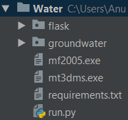
This software has been created by using a micro-framework based on Python, called Flask and for the proper management of the dependencies in this project, a virtual environment has been created. The front end has been designed using HTML, CSS and bootstrap, the back-end is being handled by the open source management system, MySQL and the integration of the front-end and back-end is done through Python(3.6.8). The interactivity of all the components have been achieved by JavaScript.

- Virtual environment folder
- Main folder (groundwater)
- Two Bash files
- run.py(main file)

- Templates (consists of HTML codes)
- Static (consists of CSS, images, JavaScript codes etc.)
- Numerical model package(consists of code for the numerical model)
- Other python files(consists of routes, initialisation and integration codes for the web platform)

The structuring of the folders have been done according to the flask application structure. This ensures that all files are stored separately, according to their functions.
Some of the important libraries used in this project are :- Pandas – for accessing the database in order to manipulate and read the data.
- Plotly, Matplotlib, Seaborn – for generating graphs, these libraries are used for visualisation of the data.
- SQLAlchemy – for abstraction of the database.
- Sklearn, scikit-learn – for data mining and machine learning.
- SciPy – scientific library for python.
- FloPy – a package to create, run, and post-process MODFLOW based models.
Please note : The original database mentioned in this documentation refers to the database that is already existing in the software.
For using this software, first make sure that you have an account. To make an account, you can click on register and enter the necessary details that are required. You can then login with your registered email id and password.
There are 6 boxes that get displayed on the ‘Groundwater quality toolboxes’. The site database model, analytical model and empirical model are complete and can be used. The optimization tool would be completed in the future.
You can begin by using the sites database model :- Create your own database by either entering all parameters manually or upload a .csv file (you can download a sample csv file for checking the format to ensure that your file can be successfully uploaded).
- You can also continue without creating your own database.
- Navigate to ‘Analysis Visualisation’ and then, to ‘All plots’ to see the visualisations available.
- Starting with the bar graph, you would be able to see that your database(in case you have created one) would be merged with the original database(already provided in the site).
- Similarly, you can navigate to the boxplot, scatterplot and histogram to visualize different types of density curves and fits for important parameters like ‘Plume length’.
- The statistical analysis page provides you with an overall description of the original database by giving the quartiles, counts, etc.
- After using this toolbox, you can move onto the analytical and empirical models.
- Read the documentation for the equation that you want to use.
- The single computation mode for each equation will require only one entry for each parameter.
- The outputs for the single computation mode will be the ‘Maximum plume length’ and a graph displaying the plume lengths in the original database and one that is calculated with the user inputs.
- The interactions for the graph can also be done via sliders, which have the most sensitive parameters.
- By changing the values in the sliders, the displayed value for plume length as well as the entry on the graph changes, making it easier for the user to visualise their results.
- The multiple computation mode for each equation allows multiple entries to be entered into the database. A separate table is created for each equation in the database.
- For using this mode, the entries for the equation can be entered manually or can be uploaded via a .csv file.
- For this purpose, please check the sample files for each parameter, to ensure that your file gets uploaded successfully.
- After creating your own database, your entries are shown along with the original database on a graph, this helps to visualize and compare all entries.
- If you wish to see only some of the entries from the original database, you can choose them from the dropdown.
For the numerical model, enter all the values of the parameters to get a ‘Maximum plume length’ according to the values entered.